Scalable Diffusion Models with Transformers

Introduction

• New class of diffusion models based on transformers, called Diffusion Transformers (DiTs).
• Show that U-Net inductive bias is not crucial for performance.
• Study the scaling behaviour of transformers with respect to network complexity vs sample quality.

Preliminaries

Diffusion Formulation

• Gaussian diffusion models assume a forward noising process which gradually applies noise to real data. \(q(x_t|x_0) = N(x_t;\sqrt{\bar{\alpha_t}}x_0, (1-\bar{\alpha_t})I\) where constants \(\bar{\alpha_t}\) are hyperparameters.

• By applying the reparametrization trick, we can sample \(x_t = \sqrt{\bar{\alpha_t}}x_0 + \sqrt{1-\bar{\alpha_t}}\epsilon_t, \epsilon_t \sim N(0, I).\)

• Diffusion models are trained to learn the reverse process that inverts forward process corruptions:

\[p_{\theta}(x_{t-1}|x_t) = N(\mu_{\theta}(x_t), \Sigma_{\theta}(x_t))\]

• Neural networks are used to predict the stats of \(p_{\theta}\).

• The reverse process is trained with the varaiation lower bound of the log-likelihood of \(x_0\) which reduces to : \(L(\theta) = -p(x_0|x_1) + \sum_tD_{KL}(q^*(x_{t-1}|x_t,x_0) \ || \ p_{\theta}(x_{t-1}|x_t))\)

• Since both \(q^* \ and \ p_{\theta}\) are Gaussian , \(D_{KL}\) can be evaluated with their means and co-variances.

• By reparametrizing \(\mu_{\theta}\) as a noise prediction network \(\epsilon_{\theta}\), the model can be trained using simple mean-squared error between the predicted noise and ground-truth sampled Gaussian noise. \(L_{simple}(\theta) = ||\epsilon_{\theta}(x_t) - \epsilon_t||^2_2\)

• In order to train diffusion models with a learned reverse process covariance \(\Sigma_{\theta}\), the full \(D_{KL}\) term needs to be optimized.

• Train \(\epsilon_{\theta}\) with \(L_{simple}\) and \(\Sigma_{\theta}\) with the full \(L\).

• New images can be sampled by initializing \(x_{t_{max}}\sim N(0,I)\) and sampling \(x_{t-1}\sim p_{\theta}(x_{t-1}|x_t)\) via reparametrization trick.

Classifier-free Guidance

• Conditional models take extra information as input such as class label c.
• The reverse process becomes \(p_{\theta}(x_{t-1}|x_t,c)\), where \(\epsilon_{\theta}\) and \(\Sigma_{\theta}\) are conditioned on \(c\).

• Diffusion sampling procedure can be guided to sample \(x\) with high \(p(x|c)\) by:

  \(\hat{\epsilon_{\theta}}(x_t,c)=\epsilon_{\theta}(x_t,\phi)+s.(\epsilon_{\theta}(x_t,c)-\epsilon_{\theta}(x_t,\phi))\) where \(s>1\) indicates the scale of guidance.

Latent Diffusion Models

• Training in high-resolution pixel space computationally prohibitive.
• Tackle with 2-stage approach:
  • Learn an autoencoderthat compresses images into smaller spatial representations with a learned encoder \(E\).
  • Train a diffusion mode of representations \(z=E(x)\) instead of diffusion model of images \(x\).
• New images generated by sampling a representation \(z\) from diffusion model and decoding it to an image with the learned decoder \(x=D(z)\).

Design Space

Patchify

• Input is spatial representation \(z\).
• First layer is “patchify:
  • Converts spatial input into a sequence of Tokens.
  • by linearly embedding each patch in the input.

DiT block design

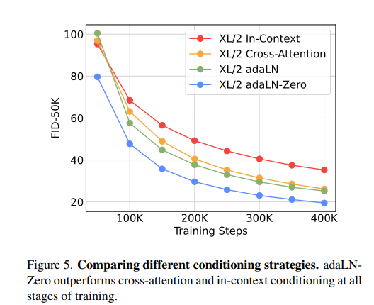
• 4 variants of transformer blocks that process conditional inputs differently:

  • In-context conditioning: Append vectors embeddings of \(t\) and \(c\) as two additional tokens in the input sequence.

  • Cross-attention block: Concatenate embeddings of \(t\) and \(c\) into a length-two sequence. Add a multi-head cross attention b/w this sequence and output of self-attention block.

  • Adaptive layer norm (adaLN) block: Use Adaptive layer normalization. Regress dimensionwise scale and shift params, \(\gamma\) and \(\beta\) from the sum of embedding vectors of \(t\) and \(c\).

  • adaLN-Zero block: Regress dimensionwise scaling parameters \(\alpha\) applied before any residual connection. Initialize the MLP to output zero-vector for all \(\alpha\), initializing the full-DiT block as identity fucntion.

Model Size

• A sequence of \(N\) DiT blocks, each with hidden dimension \(d\).
• 4 configs: DiT-S, DiT-B, DiT-L DiT-XL.

Transformer decoder

• DiT gives a sequence of image tokens.
• We need to convert it into output noise and diagonal covariance prediction.
• Use standard linear decoder.
• Apply final layer norm and linearly decode each token into a \(p\times p\times 2C\) tensor, where \(C\) is the number of channels in the spatial input.
• Finally rearrange the decoded tokens into original spatial layout to get predicted noise and covariance.

Experimental Setup

• Models named according to config and latent patch size \(p\), example, DiT-XL/2 refers to the XLarge Config and p=2.

Training

• Train at 256 x 256 and 512 x 512 resolution.
• Imagenet Dataset
• Initialize final layer with zeros and standard weight initialization techiniques from ViT otherwise.
• AdamW.
• Constant learning rate of \(1\times10^{-4}\), no weight decay and batch size of 256.
• Data augmentation - Horizontal flips.
• Maintain exponential moving average(EMA) of DiT weights over training with a decay of 0.9999.

Diffusion

• Off-the-shelf pre-trained variational autoencoder model from Stable Diffusion.
  • Downsmaple factor of 8.
• Retain diffusion hyperparameters from ADM (Ablated Diffusion Model).
  • Use \(t_{max}=1000\) linear variance schedule ranging from \(1\times10^{-4}\) to \(2\times10^{-2}\).
  • ADM’s parameterization of \(\Sigma_{\theta}\)
  • ADM’s method for embedding timesteps and labels.

Evaluation

• Frechet Inception Distance (FID)

Experiments

DiT block design

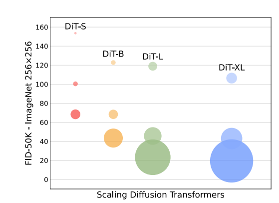
Scaling model size and patch size

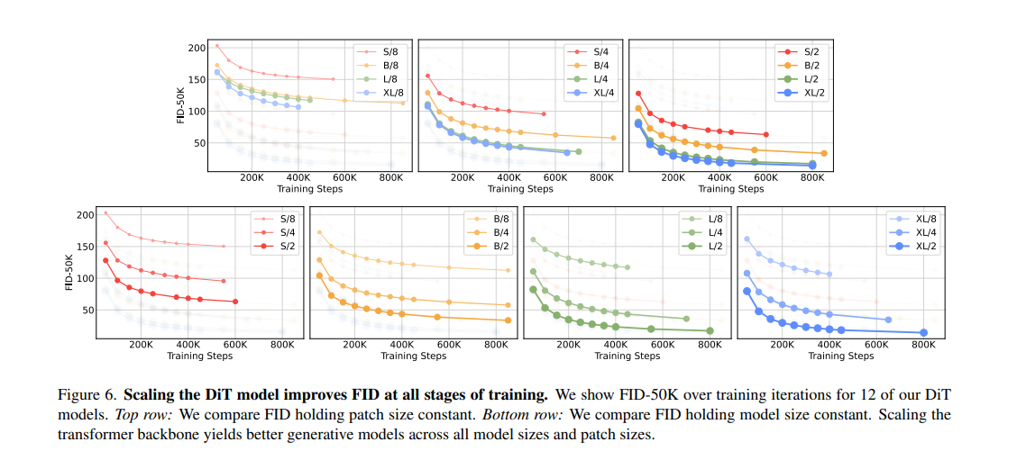
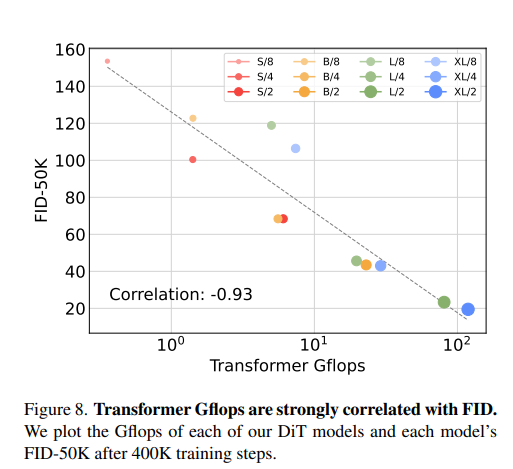
DiT Gflops

• In the exp where model size is constant and patch is decreased, total params are effectively unchanged.
• Only Gflops are increased.
• Indicating that saling model Gflops is key to improved performance.

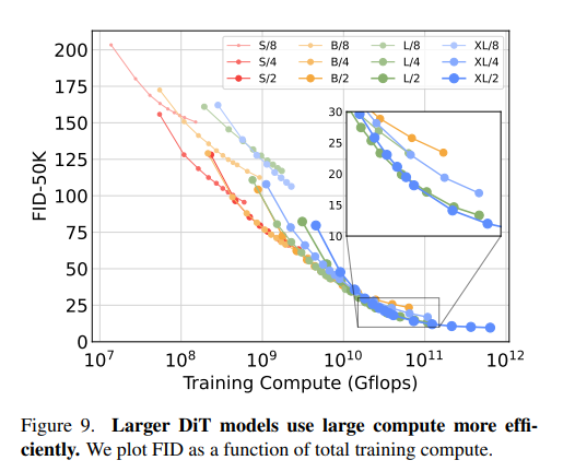
Larger DiT models are more compute-efficient

• Training compute of model:
  • Gflops . batch size . training steps . 3
  • factor of 3 because backwad pass is twice as heavy as forward.
• Small models even when trained longer, eventually become compute-efficient.

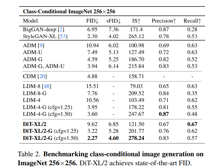
Comparison with State of Art

256 x 256 Imagenet

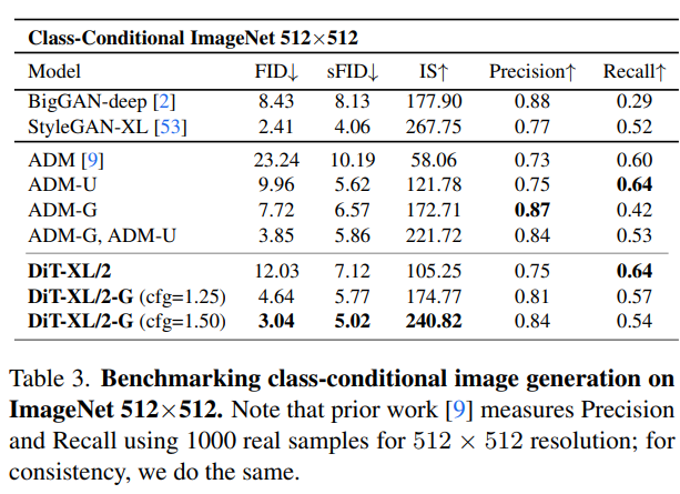
512 x 512 Imagenet